Subsurface Sensing Explained: Permittivity, Pulse Design and the Hyperbola at the Heart of GPR

Ask a hardware engineer how to locate an impedance discontinuity in a long cable and the answer is almost always reflectometry: launch an edge, watch what returns, and convert round-trip delay into distance. Ground penetrating radar (GPR) is that same measurement discipline with the dielectric beneath your boots standing in for the coax. Replace a controlled 50 Ω transmission line with layered soil, aggregate, moisture and voids, and the problem gets harder — not because the physics changes, but because the "line" is lossy, inhomogeneous and impossible to probe with a scope probe.

This primer lays out the transferable ideas behind GPR: why permittivity sets wave speed, how speed becomes a depth axis on a display, which front-end decisions decide whether a faint deep echo survives, and what to expect when the ground itself fights back. The framing is deliberately general technique rather than product review, because every one of those concepts also applies to TDR bench work, ultrawideband sensing and materials characterisation.

What the instrument actually measures is contrast

A radar unit does not photograph objects. It registers the boundary where one material's relative permittivity ends and another's begins. A buried pipe appears because pipe wall, internal air or water, and the surrounding moist soil form a short stack of dielectric steps; a clean void in imported fill can generate as strong a response as many metal targets. Reflected amplitude scales with the size of the permittivity jump, so a target whose properties match its surroundings can vanish completely while a subtle bedding plane dominates the whole trace.

That is why the method is best described as an RF boundary detector. It is not x‑ray vision for the ground: nothing is imaged as a silhouette. Echoes exist only where electrical properties change, and everything else on the screen is geometry, calibration and inference.

Wave speed, travel time and the depth axis

Relative permittivity controls propagation velocity — higher permittivity means slower wave travel — and the two-way time measured by the receiver is converted into depth only after a velocity has been assumed or independently derived. Every practical trick, from estimating velocity out of the curvature of a diffraction hyperbola to reading a time-to-depth scale on a handheld console, rests on that one relationship. Air is close to free-space velocity, dry soil, concrete and asphalt slow the wave moderately depending on density and composition, and saturated material climbs sharply, which is exactly why wet ground strengthens reflections while shrinking the usable window.

Coupling belongs in the same discussion. Ground-coupled antennas push energy directly into the medium and buy depth; air-coupled designs trade reach for resolution and portability, which suits bridge decks, road surfaces and other scenarios where contact is impractical.

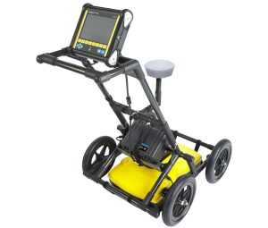
Figure 1: the Radiodetection LMX200 GPR system, shown with a high-resolution display screen and integrated GPS antenna. Source: Sensors & Software.

From isolated profiles to georeferenced models

A single radar trace answers "what is 0.8 m below this spot". Positioning is what upgrades the answer to "what is below this point on the site plan". Linking every emitted radar pulse to real-world latitude, longitude and elevation turns disconnected subsurface profiles into geographically referenced 3D spatial models that can be re-visited months later.

Conventional setups lean on mechanical measuring wheels, which slip and drift on rough terrain and oblige crews to paint manual grid lines across the working area. High-precision GPS — real-time kinematic (RTK) in particular — frees survey teams to walk or drive freeform paths, automatically corrects radar depth profiles for uneven ground topography, and exports exact utility locations into GIS, CAD or Google Earth for long-term relocation and excavation safety planning.

Material behaviour at a glance

Medium	What it does to the wave	Field consequence
Air, voids, hollow layers	Near full speed; large contrast against soil	Sharp echoes — voids read like discrete targets
Dry soil, concrete, asphalt	Moderate slowing, low loss while dry	Best-case medium; rebar and duct detail comes through
Water and saturation	High permittivity, wave crawls, strong reflection	Wet soil can overwhelm a survey and cut depth range
Metal	Extreme contrast, essentially total reflection	Bright signature plus shadowing and multiples underneath
Clay, saline or conductive ground	Aggressive absorption and conductive loss	Energy dissipates; useful echoes may disappear

Centre frequency: the depth-versus-resolution bargain

Published field guidance usually quotes a penetration band of roughly 0.3 to 30 m across all soil types, with the antenna frequency and the geology jointly deciding where a job lands inside that window. Gigahertz-range radar resolves millimetre-scale features and is the right tool for scanning rebar in concrete or mapping shallow structures — but those waves are absorbed quickly, so penetration drops below a metre. Lower-frequency systems reach tens of metres and expose large formations such as bedrock layers; general reference material for environmental survey work puts deep, low-frequency investigation around 15–20 m at a spatial resolution of only 0.5–1.5 m, which is enough for stratigraphy but not for small services. Fine pipes blur away and you are left with the bigger picture.

The working rule is to select the highest antenna frequency that still reaches the target depth, and to re-select it per line rather than per project, since ground conditions change across a site. Because GPR operates in ultrawideband ranges, spectrum regulations and licensing must be settled before deployment.

Inside the instrument: impulse and SFCW front-ends

An impulse GPR system is assembled from segments that each address one difficulty of probing underground. Read the list below as a generic wideband receiver design brief — the same constraints show up in any pulsed RF measurement.

• Transmitter. The front end fires sub-nanosecond, high-voltage pulses into an ultrawideband antenna, commonly a bow-tie or tapered slot design. Pulse purity matters because ringing or lingering oscillation blurs the radar's timing, so engineers shape clean, sharp impulses instead of simply maximising radiated energy.
• Receiver. Soil attenuation is exponential: shallow reflections can be overwhelmingly strong while deep echoes arrive as faint microvolt signals. A high-dynamic-range front end has to capture both extremes without distortion, which is where gain control, compression and careful filtering are won or lost.
• Time-domain sampling. Fleeting pulses demand clever timing. Equivalent time sampling (ETS) reconstructs picosecond-scale events on a manageable hardware budget, while high-speed ADCs paired with MCUs or DSPs provide direct digitisation in modern designs.
• Frequency domain (SFCW). Not every system is impulsive. Stepped-frequency continuous wave radar sweeps through frequencies with direct digital synthesizers (DDS); in that scheme the tone set behaves like a synthetic probe whose inverse Fourier transform yields a high-resolution range profile. SFCW buys fine frequency control, per-tone energy management and easier digital processing, while impulse systems retain the edge in raw time sharpness — a genuine either/or depending on the application.

Signal processing: the hyperbola is information, not artifact

Data starts as the A-scan, one trace of signal amplitude against time delay at a single position. Stacking A-scans as the antenna travels produces the B-scan, the two-dimensional cross-section operators actually look at. Inside those sections, point targets such as buried pipes consistently appear as upside-down hyperbolas.

The curve is geometry, not a fault. As the antenna approaches the target the travel path shortens, directly above the target it is at its minimum, and moving past it the path lengthens again; that changing slant-range distance is exactly what draws the hyperbolic signature surveyors use to separate compact objects from broad subsurface layers. The apex marks the target's true location, and the flare of the arms is what lets velocity be back-calculated — which is why interpreters treat the shape as a feature to be mined rather than noise to be removed.

Pre-processing therefore works outward from the raw record: baseline subtraction and background filtering suppress system ringing and surface clutter, gain staging recovers deep energy, and migration algorithms collapse the diffraction flare toward a point, sharpening the image so C-scans and full 3D reconstructions can be built from stacked lines.

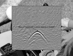
Figure 2: a line-scan GPR display of signal amplitude versus depth and position. Conical radar emission creates a characteristic hyperbolic reflection for point targets such as pipes, rocks and roots, with the target's true location marked by the apex of the hyperbola. Source: Author.

Bench-scale radar: practising the physics without a survey crew

Modern radar technology is accessible enough that hobbyists and bench engineers can explore the same principles. Compact ultrawideband (UWB) radar chips, low-cost vector network analyzer modules such as the NanoVNA, and software-defined radios (SDRs) make it possible to experiment with frequency-modulated continuous wave (FMCW) or stepped-frequency continuous wave (SFCW) radar on a workbench — hands-on observation of how signals reflect, attenuate and reveal boundaries, with no industrial-scale equipment.

A representative instrument is the VNA6000 (NanoVNA V3), a two-port 6 GHz vector network analyzer module delivering performance comparable to higher-end professional instruments in a small, portable form factor. Step a tone set across that bandwidth and transform it into the time domain and you have, in effect, a laboratory SFCW rig: you can watch directly how windowing choices, gate placement and residual ringing reshape the reconstructed range profile — the same failure modes a field crew fights on a real line.

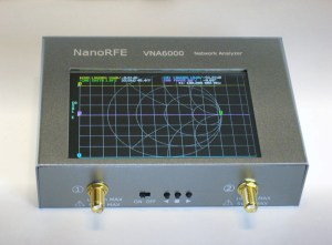
Figure 3: the VNA6000 (NanoVNA V3), a two-port 6 GHz vector network analyzer module delivering performance comparable to higher-end professional instruments in a small, portable form factor. Source: NanoRFE.

Simulation closes the loop. Open-source, FDTD-based radar modelling tools let you build a synthetic buried target, generate its hyperbola and then test your own interpretation against a known answer — a useful habit before trusting any real dataset.

Where GPR stops working

The limits are physical rather than commercial. High clay content soils absorb signals aggressively, saltwater intrusion creates strong conductive losses, and hyper-conductive soils scatter energy so severely that useful echoes vanish. These edge cases are a reminder that GPR success depends on the physics of the medium being probed, not on the price of the instrument. Where loss dominates, plan shallower objectives, lower frequencies, denser ground truth and confirmation by vacuum excavation before any dig.

Common misconceptions

• "Radar images objects." It detects dielectric discontinuities. A target electrically similar to its surroundings can be genuinely invisible.
• "Lower frequency is simply better because it goes deeper." Depth without resolution cannot find a 50 mm service; the trade-off is won by matching frequency to the objective, not by maximising reach.
• "Every hyperbola is a pipe." Tree roots, voids and soil heterogeneity can mimic the same signature; only the apex, context and verification identify it.
• "The depth readout is measured." It is computed from an assumed or derived velocity, so a wrong permittivity assumption shifts the whole profile.
• "GPS makes grid lines obsolete for every site." RTK removes painted grids on open ground, but canopy, tall walls and urban canyons still cause fix degradation that crews must manage.
• "Bench experiments are a toy." The reflection, attenuation and timing behaviour seen with an SDR or a small VNA is the same chain of cause and effect as in a full survey system.

Field workflow checklist

1. State the target: what has to be found, at what nominal depth, at what required resolution.
2. Characterise the ground first — clay content, salinity, moisture, expected loss — and accept that some sites are hostile.
3. Pick the highest antenna frequency that still reaches the target, and re-evaluate it per line.
4. Confirm ultrawideband spectrum compliance and any licensing needed for the deployment region.
5. Choose coupling: ground-coupled for depth, air-coupled for resolution and speed of travel.
6. Set up georeferencing, record control points, and verify RTK fix quality before acquiring.
7. Calibrate velocity on a known target or a hyperbola flare, not on a datasheet number.
8. Acquire a background or air scan so ringing and surface noise can be subtracted later.
9. Process in order: DC/baseline removal, gain, filter, migration — then interpret.
10. Flag ambiguity: roots, voids and layering, and schedule potholing or vacuum excavation to confirm.
11. Export positions to GIS or CAD so the record survives the crew leaving site.

FAQ

Is GPR the same technology as airport X-ray screening?

No. GPR emits non-ionizing ultrawideband radio-frequency energy and listens for reflections from dielectric boundaries; it is not x‑ray vision for the ground, and it forms no silhouette of a buried object. Interpretation is inference from echo geometry.

How is a depth number actually produced?

From velocity and time. Permittivity sets wave speed, depth equals speed multiplied by two-way time divided by two, and the A-scan's time axis becomes a depth axis only once a sensible velocity has been assumed or derived from the data.

Can radar find a non-metallic pipe?

Often, yes — the target needs contrast, not conductivity. A plastic pipe registers through the step between wall, contents and surrounding soil, and moisture or backfill differences frequently strengthen that contrast.

Why does a wet week ruin a previously good survey?

Water has high permittivity, so waves slow and reflections strengthen, while saturated ground also increases loss. Strong shallow echoes can swamp the record and shorten the effective penetration depth.

Which architecture should an electronics team prototype first, impulse or SFCW?

If you need maximum time sharpness and simple pulse timing, impulse. If your workflow is already DSP-heavy and you want fine frequency control with straightforward digital processing, SFCW with a DDS-driven sweep is the easier path to reproduce on a bench.

Do I need industrial equipment to learn this?

No. A NanoVNA-class module, an SDR and a couple of reflectors demonstrate the whole chain — launch, propagate, attenuate, reflect, digitise, transform — and let you practise the reading skills that field data demands.

Takeaway: read the ground as an RF engineer

GPR is easiest to master when it is treated as an ordinary wideband measurement problem with a very unruly test fixture. The boundary, the velocity, the pulse, the dynamic range and the geometry of the returned curve are all things an electronics engineer already reasons about daily; the subsurface merely adds attenuation, heterogeneity and a great deal of interpretation risk. From professional survey teams mapping infrastructure to hobbyists running SDRs on a workbench, the same principles of echoes and discontinuities apply — and the ground stays generous with hidden boundaries for anyone willing to model them properly.

The practical next step is small: build a bench reflectometry rig, model one buried target in open-source FDTD software, then re-read a public GPR section with the hyperbola's apex in mind. That habit — questioning the assumed velocity before trusting the depth — transfers far beyond radar, into every measurement where a signal returns changed and you have to explain why.